Hey all! Whether you’re studying or here for fun, I’ll walk you through a Perfect Substitutes Utility Maximization problem. You can see similar articles here.
We’ll focus on core concepts throughout and the intitution behind the steps. Leave a comment if you get confused!
Say we have a consumer who likes Coke C just as much as they like Pepsi P. We can denote this consumer’s utility function for these two goods as U(C,P) = C + P
U(C,P) means that U (“utility”) is a function of C and P. C and P is the form that function takes, like, say, f(x) = 3x. So, if consumer drinks 2 Cokes and 1 Pepsi, they get a utility of 3, while if they drink 3 Pepsis and 1 Coke, they get a utility of 4.
We can immediately notice a few things from this utility function. First, the goods are perfect substitutes—our consumer is indifferent to drinking a Coke versus a Pepsi. Second, the indifference curves are going to be linear. A utility function with an exponent (say, U(x) = x²) will change its slope over time. The form C + P simply adds the quantity of goods consumed (this applies to any numeric coefficient added to either variables, generalized to xC + yP), meaning the slope is constant, thus producing a linear curve. Third, the marginal rate of substitution is constant. We can infer this from the goods being perfect, linear substitutes, as the MRS describes the willingness of a consumer to replace one good for another. Since we know our consumer is indifferent to Coke versus Pepsi, they are willing to exchange at a 1:1 rate, but no less (they will not trade 1 Coke for 0.9 Pepsis).
With these observations in mind, we can plot our consumer’s preference for Coke and Pepsi:

The red line represents an indifference curve for a fixed level of utility U-bar. U-bar can be any number: 10, 50, 100, etc. At any point along the line, the U-bar level of utility is produced. For example, say our consumer has is buying 12 sodas to consume this week (we’ll get to the budget line soon), and she’s picking from a bin with infinite Cokes and Pepsis. Because she’s buying some combination of 12 Cokes and Pepsis, her utility will be 12, and so U-bar is fixed at 12:
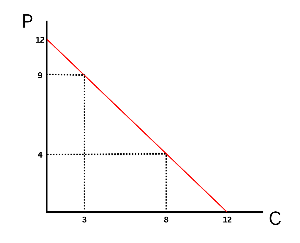
Whether she purchases 3 Cokes and 9 Pepsis, 8 Cokes and 4 Pepsis, or picks any other combination of goods along the line, she is perfectly indifferent because she gets a “total” utility of 12 regardless. As in the previous image, the slope of this line is 1 because the MRS is 1, meaning she’s willing to exchange Coke for Pepsi at a 1:1 rate.
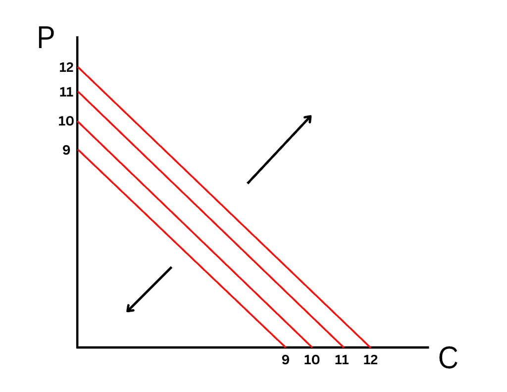
An infinite number of indifference curves exist to match the infinite number of consumption bundles, or U-bars, that exist. For example, our consumer might (theoretically )have the option to buy just 1 Coke or Pepsi, or 100, or 10,000, or 1,000,000.
So, how do we know how much Cokes and Pepsis our consumer will buy?
Typically, in a problem of this sorts, you’ll be given the prices of the goods and the budget (income) of the consumer. In this example, let’s say a Coke costs $2, a Pepsi costs $1, and our consumer has $60 to spend.
The amount of our consumer spends must equal the quantities of the goods she buys times their price. Generally, this takes the form:
P(x)*x + P(y)*y … + P(n)*n = Y
So, the price of good X times the quantity of good X consumed, added to the quantities of all other goods consumed times their prices, equals one’s budget. In our example:
2C + 1P = 60
So, our consumer could purchase 60 Pepsis for $60, 30 Cokes for $30, or some combination thereof, to set the left side of the equation (her spend) to the right side (her budget).
We can now add this budget constraint line to our graph by calculating the intercepts and drawing a linear line to connect them. To balance the equation, when P = 0, C = 30, and when C = 0, P = 60. So, let’s add points at (30, 0) and (0, 60), and connect these points with a line:
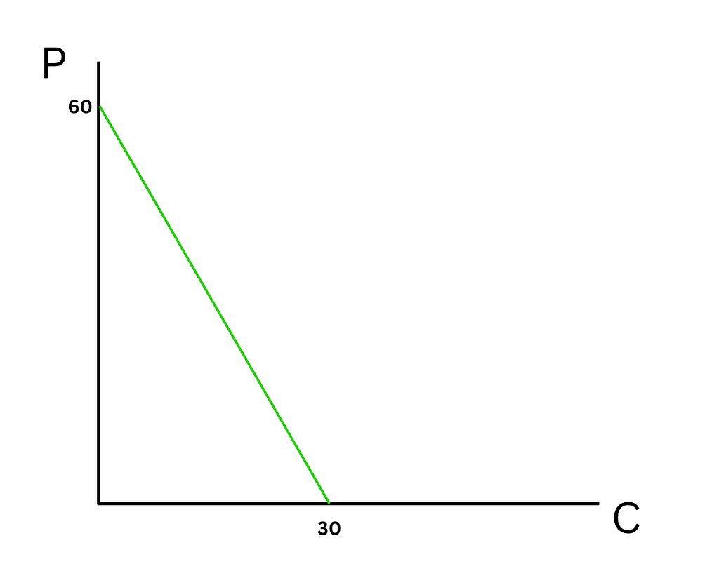
So, we have two parts: the budget constraint line, and an infinite number of indifference curves. Let’s put those two parts on the same graph:
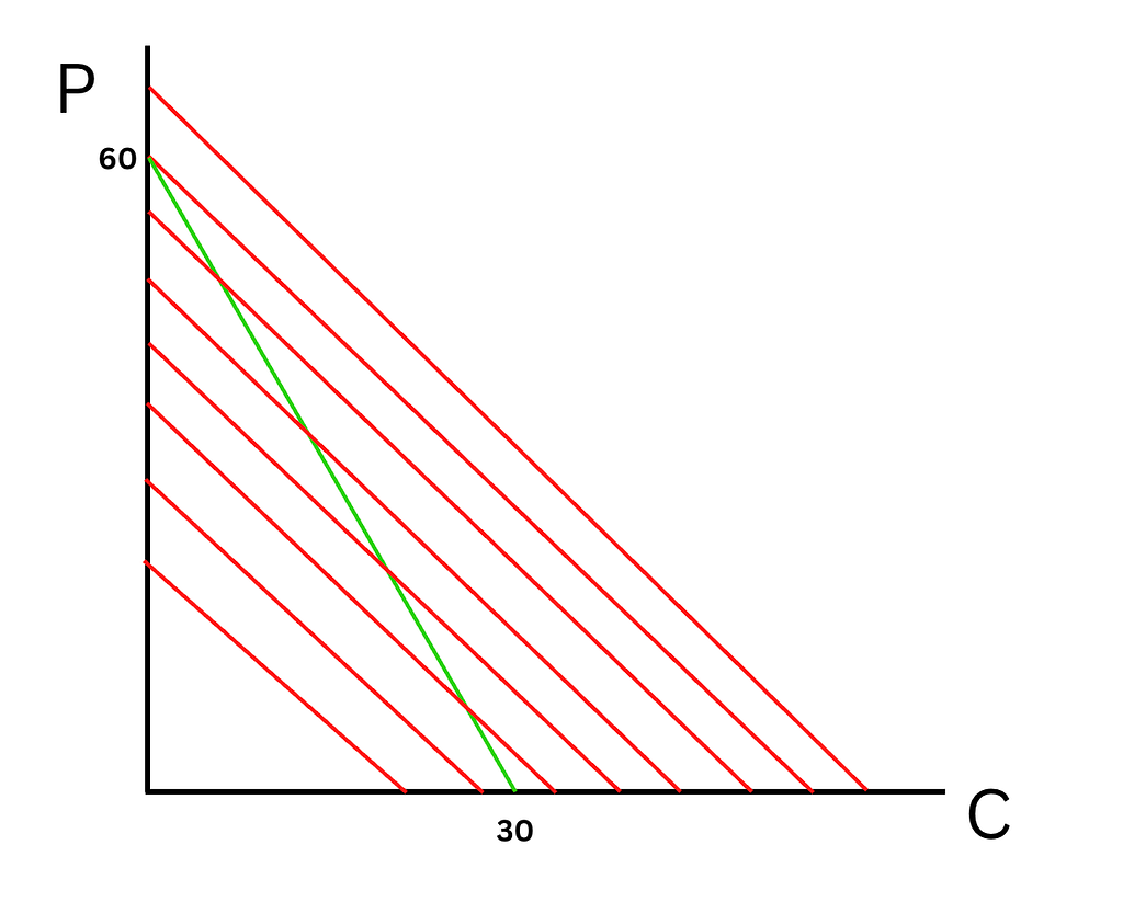
Conceptually, our consumer must choose a point on the green line (the budget constraint) because she doesn’t have more money. Remember that each indifference curve represents a different, fixed level of utility. We also know that consumers, naturally, want to maximize their utility (more utility is inherently better than less).
That leads to the question: what point on the budget constraint line maximizes the utility for our consumer?
We can calculate it, since we know U = C + P. At the x-intercept, U = 30 + 0 = 30. Higher up on the budget constraint line, say when 15 Cokes are consumed, U = 15 + 30 = 45. At the y-intercept, U = 0 + 60 = 60. So, the higher we go on the budget constraint line, the more utility we get, with the maximal utility at the y-intercept.
Visually, this occurs because indifference curves represnt higher levels of fixed utility as we shift rightward on our graph (away from 0). I’ll highlight the highest level of utility (the farthest away from 0) that touches a point on the budget constraint line:

The highest indifference curve that the budget constraint touches is where the consumer will allocate resources to maximize their utility. This point (0, 60) lines up with our utility calculations, whereas U = C + P, so plugging in (0, 60) we get U = C + 60 = a utility of 60.
Here’s a shortcut: if you see a utility function with perfect substitutes, and the prices of the goods are different, you will always get a “corner solution”—a solution hitting an intercept on the graph. Intuitively, this occurs because you get the same “pleasure” or utility from each good, but one is cheaper to acquire than the other.
To calculate the MRS for this problem, we can note that MRS equals the marginal utilities of each good, so we can take the partial derivative of the utility function with respect to the X-axis good divided by the partial derivative of the utility function with respect to the Y-axis good:
MRS = MUc/MUp = (∂U/∂C)/(∂U/∂P) given U = C + P
Thus, the MRS equates to 1/1 = 1. This is a straightforward way to calculate the slope of the indifference curve, as we know the slope is -1 (-MUc/MUp).
Finally, note the price ratio (MRT), or -Pc/Pp, which equates to (-2/1), or -2. This is the slope of the budget constraint line (-60/30 = -2).
Leave any questions in the comments! Check out my other articles on economics here (useful for studying, or just learning).